Influences of Multi-scale Built Environments on Commuting Carbon Emissions — Case Study of Xi'an

Role: Participant / National College Student Innovation and Entrepreneurship Training Programme (Country-level)

Mentors: Prof. Xiaoyan Huang

Jun 2022 – May 2023

Overview

Using a dual-anchor (residence + workplace) framework and a cross-classified multilevel model on 965 commuters in Xi'an, this study measures commuting CO₂ as distance × mode-specific emission factors × traffic-condition weights and tests income heterogeneity; we find workplace contexts explain most variance, with higher parking density and higher job accessibility around workplaces associated with higher emissions, while bus-stop abundance and metro presence near workplaces reduce emissions, and living farther from the city center raises emissions; emissions are highly concentrated (top 10% generate ~67% of commuting CO₂) and effects are generally stronger for middle-to-high-income commuters, implying policy levers should prioritize workplace-side transit investment and parking management alongside income-sensitive targeting.

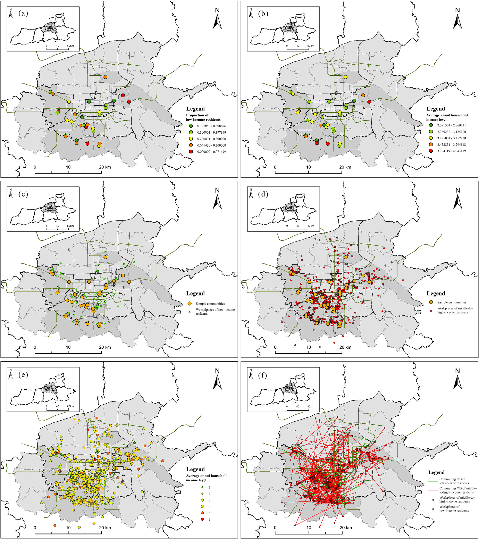Spatial distribution of LI vs. MHI residences and workplaces in Xi'an; OD lines and community-level income

Introduction

Urban commuting CO₂ in dense cities is jointly shaped by the built environment (BE) around both residences and workplaces. This study asks:

How do residential- and workplace-area BE jointly affect commuting CO₂?
Do these effects differ by income?

We implement a dual-anchor approach and explicitly test income-based disparities.

Methodology

Data & Sample

A stratified household travel survey in Xi'an (Sept–Nov 2021) yields 965 employed commuters with demographics, attitudes, preferences, perceived BE, and one-day travel diaries. Income is discretized as annual household income (AHI): LI (≤ CNY 60,000) and MHI (> CNY 60,000).

Outcome: Weighted Commuting CO₂ (WCE)

For commuter $i$ using mode $n$ :

WCE_i = D_i \times F_n \times C_i

where $D_i$ is residence–workplace distance, $F_n$ is the mode-specific emission factor, and $C_i$ is a traffic-condition correction determined by urban zones. Non-motorized modes are set to zero.

Table A. Mode-specific CO₂ emission factors (used in $F_n$ )

Mode	Emission Factor (g CO₂/km)
Private car / Taxi	233.1
Urban bus	26.0
Coach	20.3
Metro	20.9
E-bike / Walk / Bicycle	0

Table B. Traffic-condition correction factors by urban zone (used in $C_i$ )

Zone	Car/Taxi Speed	Car/Taxi Weight	Bus Speed	Bus Weight
Inside the city wall	19.05	1.71	15.76	1.65
City wall–2nd Ring	20.99	1.54	17.36	1.51
2nd Ring–Ring Expwy	29.84	1.06	24.68	1.04
Outside Ring Expwy	31.50	1.00	26.05	1.00

Explanatory Variables: Dual-Anchor Built Environment

We measure BE around residence and workplace using a 15-minute cyclist circle and the 5D framework (Density, Diversity, Design, Distance to transit, Destination accessibility).

Land-use mix (LUM) via entropy:

LUM_i = -\frac{\sum_a p_a \ln p_a}{\ln N}

where $p_a$ is the share of land-use class $a$ in region $i$ .

Job accessibility index (JAI) at Jiedao scale:

JAI_i = \frac{W_i + \sum_{j=1}^{S} \frac{W_j}{d_{ij}^2}}{WP_i}

where $W$ is job supply, $WP$ is working-age population, and $d_{ij}$ are centroid distances within 4 km.

Transit variables: bus-stop count and a binary metro presence (≥ 1 station) within each circle.
Design includes parking-lot density.
Destination accessibility includes distance to city center (Zhonglou), nearest commercial facility, and grade school.

Modeling: Cross-Classified Multilevel Model (CCMM)

Let commuter $i$ live in residence community $r$ and work in workplace community $w$ .

Level-1 (individual):

WCE_{irw} = \phi + \alpha_r + \alpha_w + \beta_S^T X_i + e_{irw}, \quad e_{irw} \sim N(0, \sigma_{irw}^2)

Level-2 (residence):

\alpha_r = \beta_R^T X_r + e_r, \quad e_r \sim N(0, \sigma_r^2)

Level-2 (workplace):

\alpha_w = \beta_W^T X_w + e_w, \quad e_w \sim N(0, \sigma_w^2)

Variance attribution (ICCs):

ICC_{res} = \frac{\sigma_r^2}{\sigma_{irw}^2 + \sigma_r^2 + \sigma_w^2}

ICC_{work} = \frac{\sigma_w^2}{\sigma_{irw}^2 + \sigma_r^2 + \sigma_w^2}

Results

R1. Distribution of emissions

Commuting CO₂ is highly concentrated: roughly 10% of commuters generate about 67% of total commuting CO₂. MHI commuters emit over 3× LI commuters on average; the disparity is driven primarily by mode choice (greater private car/taxi share), not distance.

Lorenz curve of weighted commuting CO₂ (67–10 pattern)

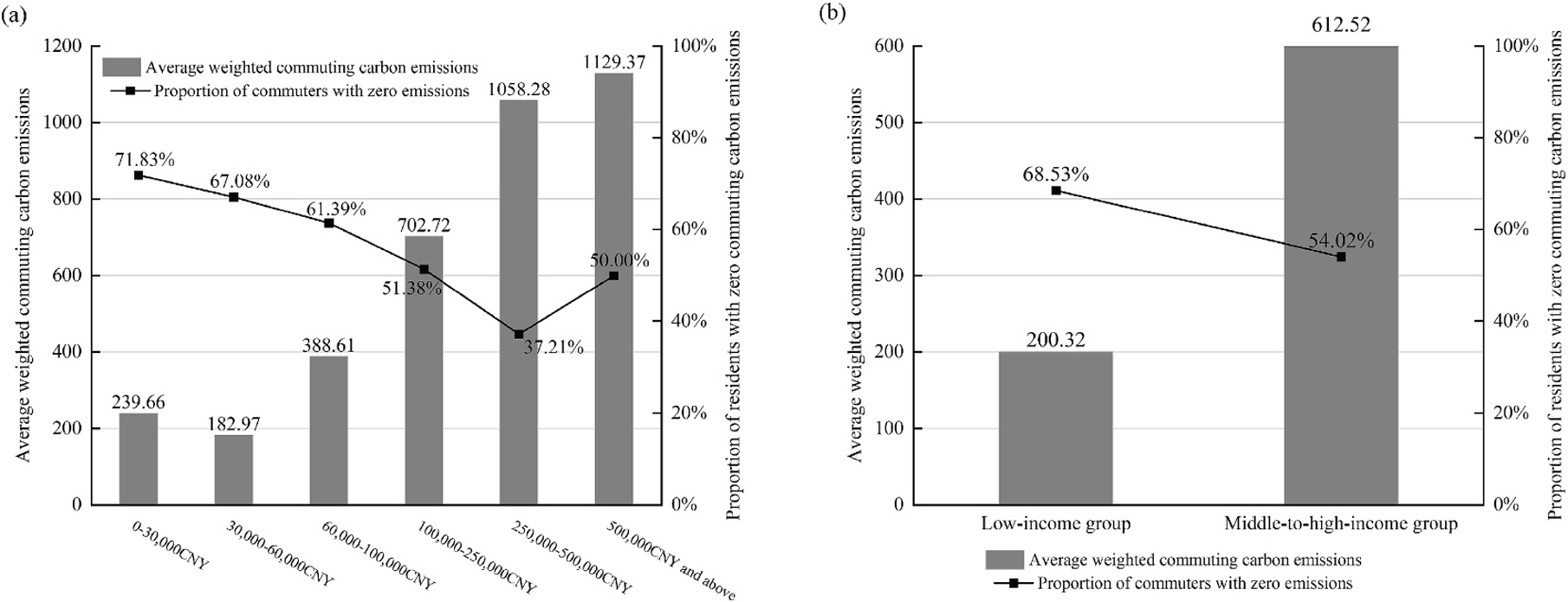Mean WCE and zero-emission share across AHI levels (LI vs. MHI)

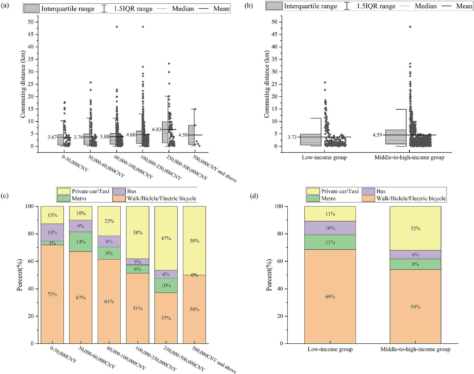Distributions of commute distance and mode across AHI levels; car/taxi share rises with income

R2. Empty CCMMs (variance decomposition)

Workplace context dominates in the full sample: $ICC_{work} = 0.731$ vs. $ICC_{res} = 0.078$ . The combined (res + work) ICC is higher for MHI (0.786) than LI (0.416), implying BE explains more for MHI commuters.

Table C. Empty-model variance components and ICCs

Group	$\sigma_r^2$	$\sigma_w^2$	$\sigma_{irw}^2$	$ICC_{res}$	$ICC_{work}$	N
Whole sample	128023.1	1192641.1	311567.3	0.078	0.731	965
LI	79081.8	85566.2	230761.6	0.200	0.216	232
MHI	130651.8	1306601.5	391232.8	0.071	0.715	733

R3. Main effects (BE → WCE)

After controls (demographics, attitudes, preferences, perceived BE), workplace-area BE shows the strongest associations:

Parking-lot density (workplace) → higher WCE
Bus-stop count (workplace) → lower WCE
Metro presence (workplace) → lower WCE
Job accessibility (workplace) → higher WCE
Distance to city center (residence) → positive: farther from center ⇒ higher WCE

R4. Income heterogeneity (interactions with AHI)

Effects generally amplify with income:

Residence distance to city center × AHI: larger reductions when living closer to center among higher-income commuters (i.e., stronger benefit of centrality at higher income)
Workplace transit × AHI: bus-stop count and metro presence reduce WCE more strongly at higher incomes
Workplace job accessibility × AHI: more positive association at higher incomes

Table D. Selected BE × AHI interactions (direction and significance)

Interaction term	Direction (MHI vs. LI)	Significance (p)
$d_{center\_r} \times AHI$	positive	< 0.05
$num_{bus\_w} \times AHI$	negative	< 0.05
$metro_w \times AHI$	negative	0.10 to 0.001
$den_{park\_w} \times AHI$	positive	* to **
$ja_w \times AHI$	positive	* to ***

Conclusions

Workplace-area BE is the primary lever: managing parking supply and strengthening workplace-proximate transit (especially metro) are robust strategies to cut commuting CO₂ in dense cities.
Income matters: many BE effects are stronger for higher-income commuters; targeted TOD and calibrated parking restraint in job centers can deliver larger absolute reductions with equity-minded transit coverage.
Residential centrality still matters: living farther from the center raises emissions; avoiding unchecked suburbanization or pursuing polycentric structures can help.